Autoclave modeling
Coupled simulation of autoclave airflow, part–tool heat transfer, and composite cure in CONVERGE.
COMPOSITE MANUFACTURING · CMSC / PURDUE · ASC 2026 PAPER 93
This project develops a coupled autoclave process model to predict composite temperature and degree of cure under a prescribed heating cycle. Thermal inertia in the tool and laminate, together with heat released by resin curing, causes the material response to differ from the chamber temperature. The model connects airflow, solid heat transfer, and cure kinetics to evaluate these differences and support future process design.
I extended the team’s existing autoclave air/heating model by adding the composite part, mold, and their thermal boundaries. I implemented the cure calculation and reaction-heat coupling in CONVERGE using established cure-kinetics and numerical-integration methods, refined model parameters against temperature measurements, and analyzed the thermal and cure histories. My work focused on model development and implementation; the experimental concept and original autoclave framework were developed by the team.
Read the paper (PDF · 1.2 MB) View the poster (PDF · 1.3 MB)
1. Model setup and formulation
The analysis evaluates part and tool thermal lag, spatial temperature variation, and the degree of cure produced by the imposed cycle. These outputs characterize the simulated material response under the specified conditions. An optimized production cycle and a demonstrated relationship to part quality remain outside the scope of this study.
1.1 Geometry and boundary conditions
The conjugate heat-transfer model resolves air circulation around the load and conduction through the solid regions. The surrounding flow and tool response therefore determine the part’s heating history. The part–mold interface assumes perfect thermal contact; contact resistance remains a subject for further study.
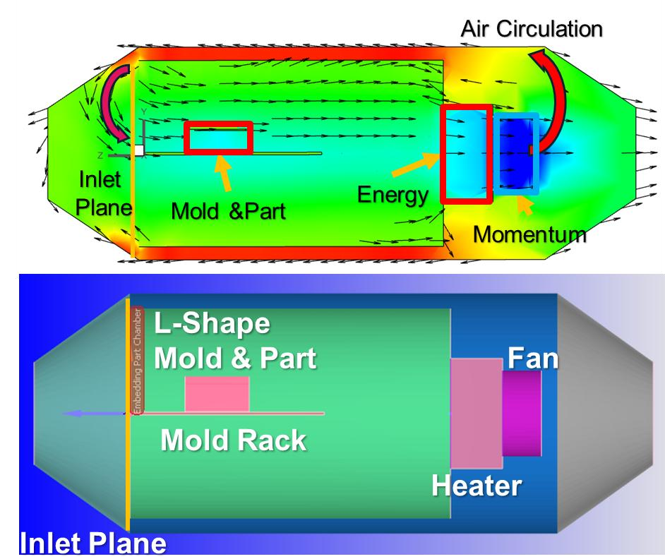
Case setup and modeling assumptions
| Element | Configuration reported in the final paper |
|---|---|
| Laminate | 10 × 10 in IM7/8552; 24 plies, [−45/0/45/90]₃s; 3 mm thick; resin mass fraction 35% |
| Tool | L-shaped aluminum 6061-T6 mold |
| Flow and heat transfer | Compressible air; SST k–ω turbulence model; PISO pressure–velocity coupling |
| Vessel | Adiabatic outer walls; airflow and heater effects represented with source terms; PID-based heating control |
| Mesh | 0.25 m base size with local refinement factors from 2³ to 2⁷ |
| Cure integration | Cellwise cure state; fourth-order Runge–Kutta (RK4), with local temperature held fixed during the cure update |
These settings describe the paper’s case. The poster lists a different laminate thickness (4 mm); its calibration figure is identified separately below.
1.2 Thermal–cure coupling
A user-defined source in CONVERGE couples the thermal solution to the cure calculation. Each composite cell retains its degree of cure, allowing the reaction state to evolve with the local temperature history.
- 01 / THERMAL FIELDRead local temperature
The CFD energy solution supplies the composite cell temperature.
- 02 / CURE UPDATEAdvance the cure state
Evaluate the adopted kinetics and integrate degree of cure with RK4.
- 03 / ENERGY SOURCEReturn reaction heat
Convert the reaction rate into a heat source in the composite energy equation.
The updated thermal field drives the next cure update, completing the feedback loop.
Temperature remains fixed within each cure update, separating the kinetic integration from the CFD solve. The rapidly accelerating exotherm requires evaluation of time-step sensitivity and the effect of this operator splitting on the transient response.
2. Numerical verification and temperature calibration
2.1 Cure-source benchmark
The numerical benchmark isolates the cure calculation in an adiabatic 1 mm³ neat-resin case: initial temperature 433 K and initial degree of cure 0.001. The fixed-step CONVERGE, MATLAB RK4, and ABAQUS UMATHT implementations use a 0.15 s time step, with adaptive MATLAB ODE45 as the reference.
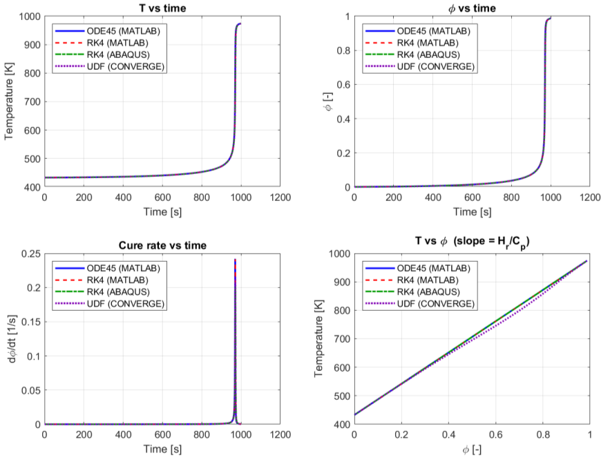
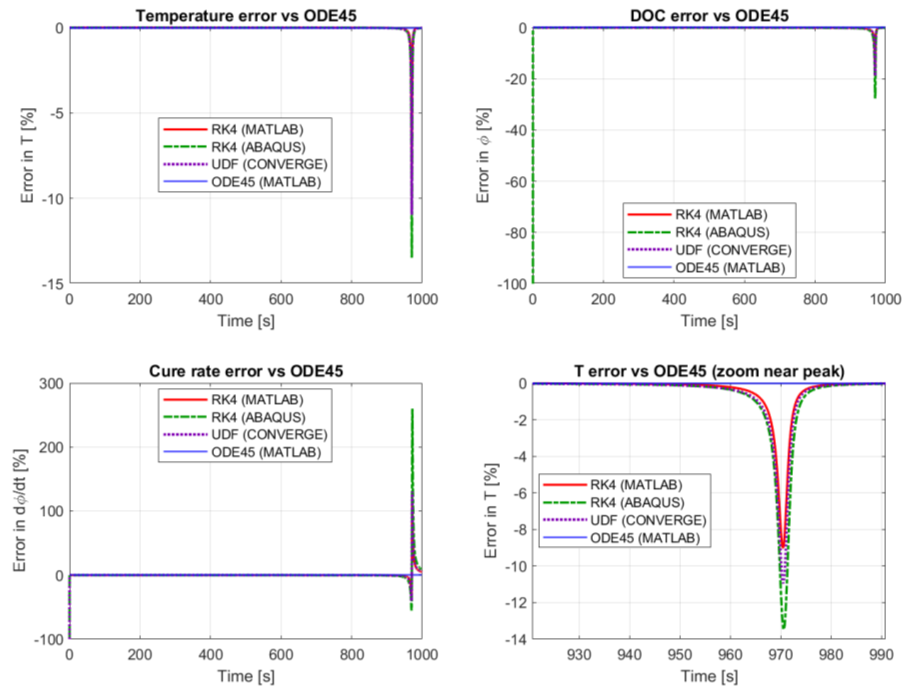
Agreement at the final state does not establish uniform agreement throughout the transient. Near the sharp temperature rise, deviations relative to ODE45 reach approximately −9% for CONVERGE/MATLAB RK4 and −13% for ABAQUS. This benchmark evaluates the numerical implementation under an idealized condition. Experimental validation of the coupled process model remains necessary.
2.2 Temperature calibration
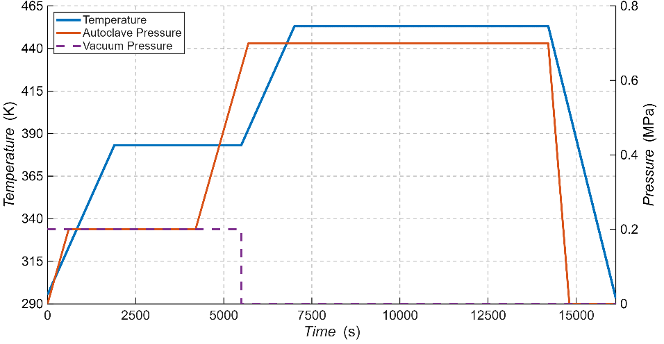
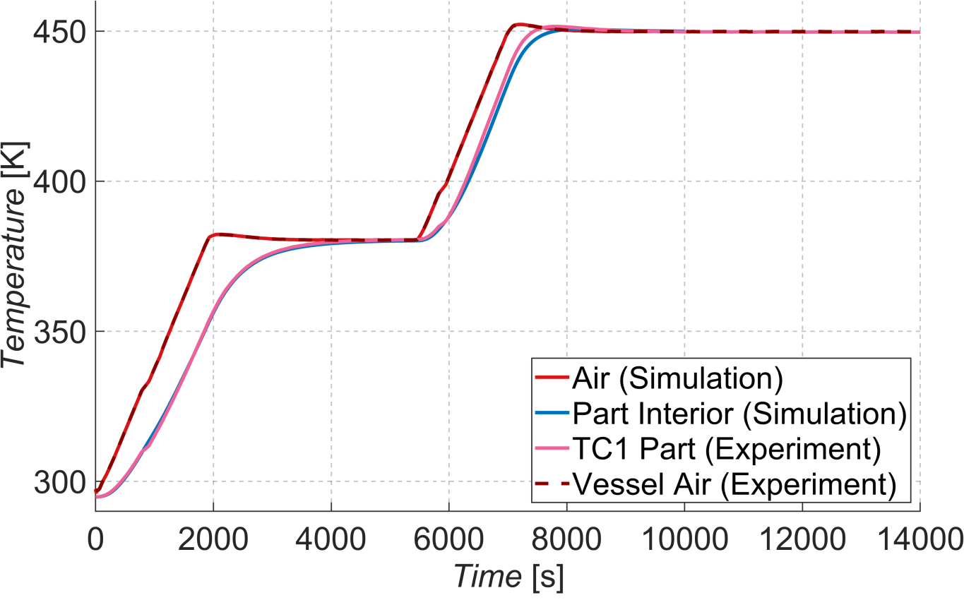
Experimental temperature histories provide the basis for parameter calibration. The poster compares part and vessel-air measurements with the corresponding simulations across the heating ramps and holds, including the thermal lag between the air and part.
3. Simulation results
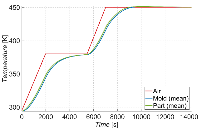
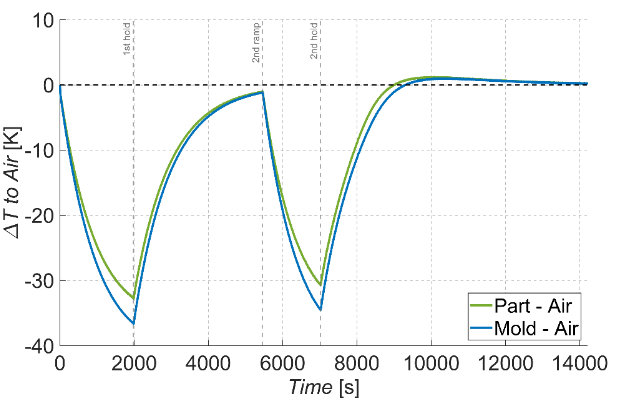
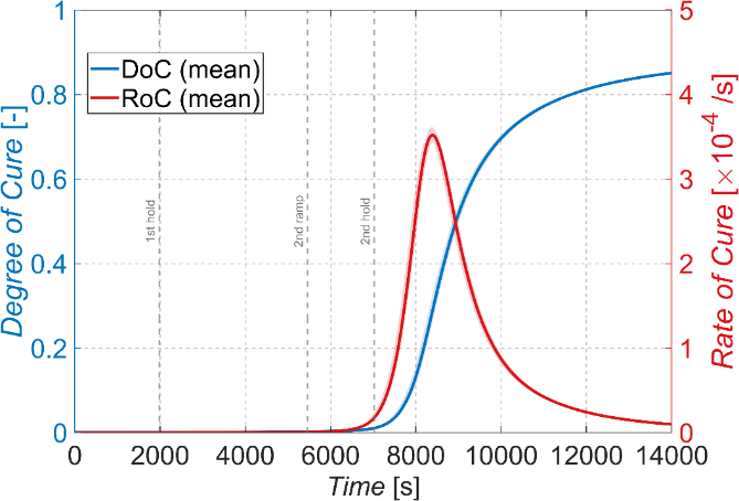
Simulation results for the paper’s material, geometry, and heating cycle; these are case-specific predictions.
3.1 Part and tool thermal lag
The largest reported lag is 33 K for the part and 37 K for the mold. Both approach the surrounding air temperature during the holds. During the ramps, the chamber temperature therefore differs substantially from the material’s thermal exposure.
3.2 Cure evolution and temperature uniformity
The predicted final degree of cure is approximately 85%. Reaction rate accelerates during the higher-temperature stage, while the final cure state reflects the full temperature history and the adopted kinetic model.
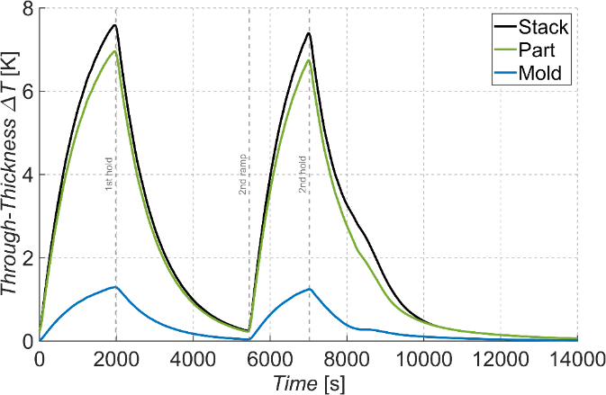
Temperature also varies spatially: the instantaneous minimum-to-maximum spread reaches about 7.5 K across the combined part–mold stack, while the part-only spread remains within 1.7 K for this case.
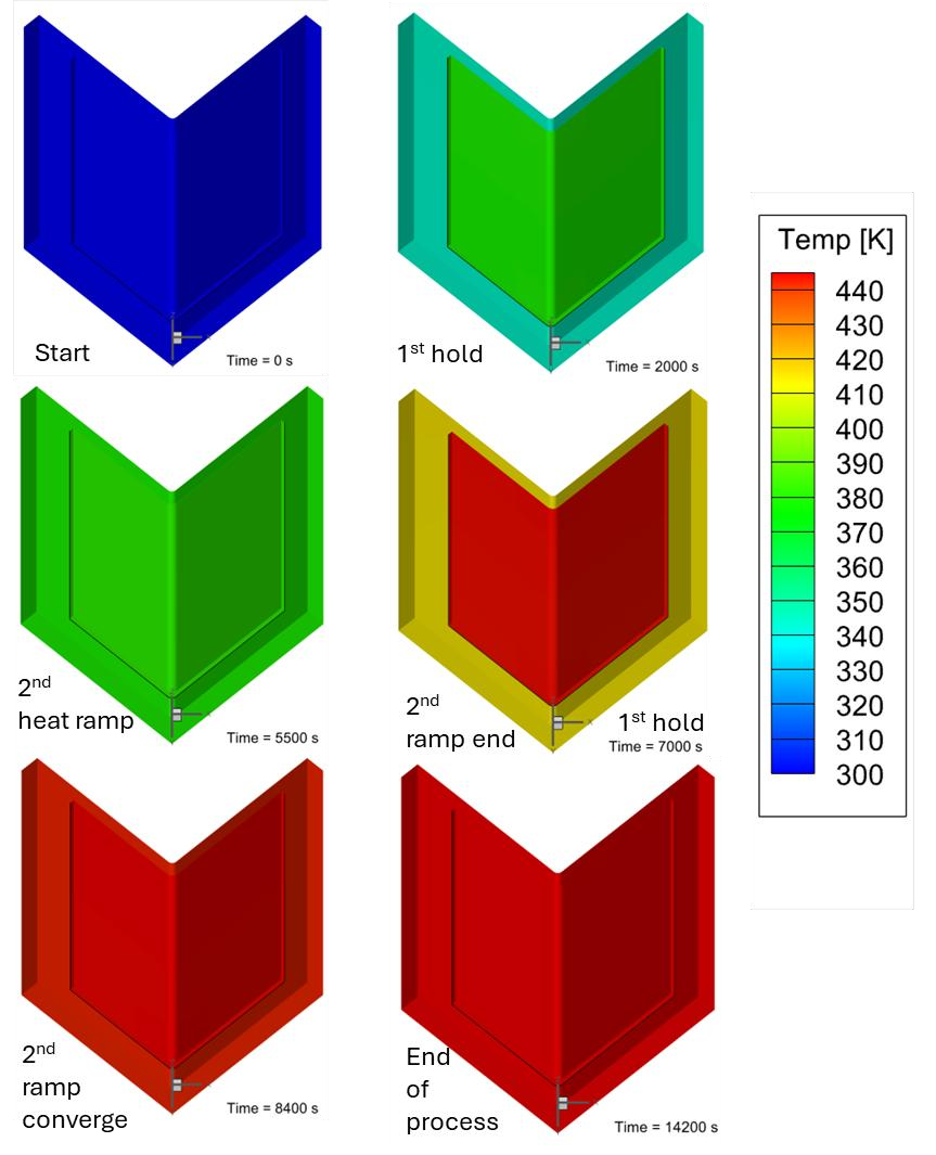
Temperature contours through the heating cycle
4. Limitations and next steps
The model links the prescribed chamber cycle to part temperature and cure. The numerical benchmark and temperature-calibration comparison support its development, while validation of the cure prediction requires measurements from a documented, matched specimen and cycle. Further evaluation should address the following:
- Cure-state measurements: retain the DSC trace, sample location, thermal history, and uncertainty so the final cure estimate can be evaluated reproducibly.
- Time-step sensitivity: resolve the rapid exotherm and quantify how operator splitting affects the transient response.
- Thermal and flow assumptions: examine contact resistance and the representation of fan/vent behavior against additional temperature measurements.
Source versions and the DSC comparison
The final paper reports approximately 85% predicted cure and describes experimental DSC/coupon validation as future work. The poster separately reports a 92.2% DSC value, a difference of about 7.2 percentage points from the prediction. The supplied materials do not establish a matched raw DSC record and test protocol for that comparison, so it is presented as a poster-reported reference rather than a completed validation result.
The paper and poster also differ in reported laminate thickness (3 mm versus 4 mm) and the written kinetic expression. This page uses the final paper for the case setup and simulation results, labels the poster calibration separately, and describes the coupling without asserting an unresolved rate equation or parameter set.
Publication and source context
A Conjugate Heat Transfer Model for Autoclave Process Simulation
Yao Sun, Hongsen Fang (Richard Fang), Lu Li, and Dianyun Zhang. ASC 2026, Paper 93.
Richard Fang is listed as Hongsen Fang in the paper’s author list. Yao Sun is identified as the presenter on the poster. The figures on this page are extracted from the supplied paper and poster, with their original axes and legends retained.
For the related instrumentation work, see AFP monitoring. The Infusion / TPS project combines multiscale infusion simulations with separate cure-dependent material development, under different assumptions and loading conditions.